How Bohr became a Top G

Modern Atomic Models Revisited

A lot changed in Physics during the 20th century.

A lot.

Our understanding of the fundamental building blocks of nature leapfrogged from that of mere undivisible balls to sub-nuclear fuzzes of probability.

In all the chaos, it is easy to neglect the humble beginnings of a new era of Physics.

One marked by competing models, countless unexplained observations and clashing egos of academic giants.

This is a how-to story on ‘rising through the ranks’ as a physicist.

Thomson’s Model

The plum-pudding model is the most ill-represented model in all of physics.

Every introductory description of the model abruptly stops at its salient feature - positively charged sphere, with electrons embedded in an undisclosed manner. The argument for the existence of positive sphere is trivial - to maintain the neutrality of the atom.

But what about the embedding scheme of electrons ?

Are they really placed as arbitraily as you have been told they are ?

In March 1904, Thomson proposed a model consisting of a uniform sphere of positive charge and a single ring of electron. The motion of each electron is governed only by its electrostatic attraction toward the center of the sphere, and by the repulsion from each of the other electrons.

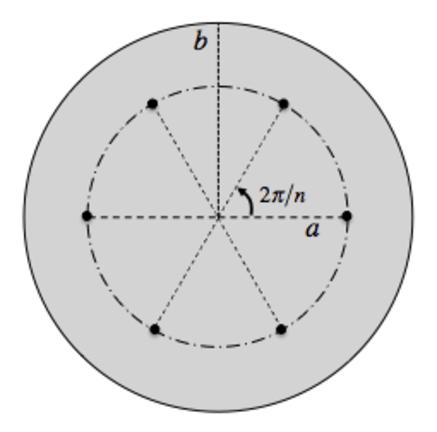
Diagram of Thomson’s 1904 atomic model. A uniform sphere of positive charge (shaded region, of radius b) contains n negative point charges arranged at equal intervals around a circle (of radius a).

(Source : Early Atomic Models - From Mechanical to Quantum (1904-1913) by Charles Baily)

Thomson had analyzed a system of n electrons (mass m and charge –e), arranged on a ring of radius a, centered within a positive sphere of radius b.

If the radially attractive force on each charge balances the net repulsive force of the other n – 1 ones, the system of charges will be in equilibrium. But, the equilibrium of a system is not sufficient for physicists to be confident. Even an upside down pencil, can theoretically exist in a state of equilibrium.

The real challenge is to comment on the stability of the equilibrium, and hence of the system.

So, Thomson, like any good physicist, considered the restoring forces on the rotating charges when slightly perturbed.

In a stable equilibrium, these electrons must oscillate about their equilibrium position. For the specific case of small displacements in the plane of rotation, these frequencies were given by the roots to a set of n equations.

Through a series of lengthy calculations, Thomson was able to show that the 2n l solutions to the equations would all be real numbers. Hence, the oscillations were indeed stable.

But, the result holds true only for n < 6 and only if rotational speed of the ring exceeded some minimum value.

Periodicity

Sadly, n = 6 gives us a mechanically unstable a ring of electrons.

Regardless of its angular velocity, the presence an additional negative charge would be required at center of the sphere to restore stability. Moreover, if the number of outer electrons was beyond 8, more and more of such interior charges would be required for the stability of the system.

Thomson thought these interior charges would arrange themselves into closed, stable orbits.

So, atoms with n > 8 must be made up of a series of concentric rings of electrons.

The number of charges would have to vary from ring to ring, with the greatest number in the outermost ring, and a decreasing number of charges occupying each of the inner rings.

The appearance of periodicity in the structure of atom convinced Thomson that the number of electrons occupying the rings and the consequent stability of the ring must closely match the periodicity of the natural elements.

Radiative Instability

The prospect seems remarkable.

Yet, like always, there’s a catch.

Classical electrodynamics predicts that any accelerated charge will radiate energy in the form of electromagnetic waves. Therefore, the kinetic energy of a system of electrons in periodic motion would be dissipated by the resulting radiation until exhausted.

Accelerated charge (electron) spiralling into the nucleus by emitting electromagnetic radiation according to classical theory.

(Source : https://chem.libretexts.org/Courses/Solano_Community_College/Chem_160/Chapter_07%3A_Atomic_Structure_and_Periodicity/7.04_The_Bohr_Model)

Thomson saw this radiative instability as a mechanism for the production of β radiation.

“… in consequence of the radiation from the moving corpuscles (electrons), their velocities will slowly very slowly diminish; when, after a long interval, the velocity reaches the critical velocity, there will be what is equivalent to an explosion of the corpuscles […] The kinetic energy gained in this way might be sufficient to carry the system out of the atom, and we should have, as in the case of radium, a part of the atom shot off. In consequence of the very slow dissipation of energy by radiation the life of the atom would be very long.”

β scattering

Up until then, Thomson’s model was only of theoretical significance.

Its predictive power was realised only when he used a modified static version of the plum-pudding model to propose several methods for determining the total number of electrons in an atom. These were based on experimental data for three different phenomena - the dispersion of light, the scattering of X-rays by dilute gases and the absorption of β-rays when traversing matter.

Each method resulted in the same conclusion - number of electrons in an atom should be on the same order of magnitude as its atomic weight.

Thomson believed the loss of kinetic energy for β-particles in an absorbing substance, and their deflection when passing through thin sheets of metal, could both be explained as resulting from a series of multiple encounters with the individual atoms in the material.

He assumed the change in energy of a β-particle deflected by a single atom would be small.

The source of this deflection would be the interactions with the uniformly distributed negative point charges modeled to being at rest. As per Thomson’s calculations, for a succession of such encounters, the number of transmitted particles would decrease exponentially with the thickness of the scatterer.

Scope for Improvement

By 1910, Thomson had generalized his earlier calculations to take into account the deflection of β-particles by encounters with both the positive and negative charge inside an atom.

However, given the limitations of the available experimental methods, the much more massive α-particles (being studied by Rutherford and Hans Geiger at the time) were better suited than β-particles for probing the internal structure of atoms through scattering experiments.

This is because the high kinetic energies of α-particles allowed for neglecting their interactions with the electrons.

Rutherford’s Model

Nagaoka’s Saturnian Model

There were several strong critics of Thomson’s model of the atom.

A significant one being Nagaoka. He rejected Thomson’s model on the grounds that opposite charges are impenetrable. So, in 1904, Nagaoka proposed an alternative planetary model of the atom in which a positively charged center is surrounded by a number of revolving electrons.

The manner in which it emulates Saturn and its rings has led to its name.

Nagaoka’s model made two predictions:

• a very massive atomic center (analogous to a very massive planet)
• electrons revolving around the nucleus, bound by electrostatic forces (analogous to the rings revolving around Saturn, bound by gravitational forces).

Both of these predictions were successfully confirmed by Ernest Rutherford.

However, other details of the model were found to be incorrect which led to Nagaoka abandoning his own proposed model in 1908.

It was crucial to mention Nagaoka before discussing Rutherford’s work, because he himself mentioned Nagaoka’s model in his 1911 paper in which he proposed the atomic nucleus.

Geiger-Marsden Experiments

The motivation behind the Geiger-Marsden experiments was an interesting phenomenon noted during the β-scattering experiments.

β-rays directed at a metal plate also resulted in radiation being emitted from the same side of the plate as the incident particles. Initially assumed to be just a secondary effect, the observed radiation was eventually shown to be comprised of primary particles that had been scattered.

So, in 1909, Rutherford asked Hans Geiger and Ernest Marsden to investigate whether this was the case for α-particles as well.

As Marsden recalls,

“One day Rutherford came into the room where [Geiger and I] were counting α-particles … turned to me and said, ‘See if you can get some effect of α-particles directly reflected from a metal surface.’ […] I do not think he expected any such result.”

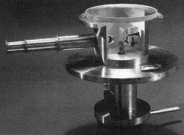
Replica of one of Geiger and Marsden’s apparatus used in a 1913 experiment

(Source : https://en.m.wikipedia.org/wiki/Geiger%E2%80%93Marsden_experiments)

By 1910, Geiger had amassed a substantial amount of scattering data by systematically varying the type and thickness of the scattering material.

He had determined that the peak scattering angle increased linearly with the stopping power of the material. This led Geiger to argue that the most probable angle of deflection was due to a single atomic encounter, and was thus, directly proportional to the atomic weight A.

Rutherford steps in

Rutherford had closely examined Thomson’s model for β-scattering.

Based of Geiger’s findings, he concluded that any large-angle deflections of an incident particle due to a continuously distributed sphere of charge would only be possible if the radius of the sphere were very small compared to the distance over which the interaction took place.

Therefore, in his 1911 paper, Rutherford discussed a possible atomic structure that he claimed, would be capable of producing such large deflections.

Unlike a uniform positively charged sphere, it contained a stationary mass of charge +Ne concentrated within a tiny volume.

His argument relied on the fact that the scattering due to electrons could essentially be ignored. This would allow him, without loss of generality, to propose that the neutrality of the atom stems from an equal amount of opposite charge spread uniformly across a larger sphere of radius R.

But more importantly, in neglecting the internal configuration of the electrons in the system, Rutherford could evade questions on the stability of his nuclear atom.

An Edge over Thomson

Thomson had relied on multiple collisions to explain β-scattering.

However, for small thicknesses, Rutherford found that the probability of a particle being scattered by a given angle by a single atomic encounter was always greater, than the probability for compound scattering to achieve the same result.

To be precise, in 1911, Rutherford estimated the average scattering angle by both the methods.

The angle for single encounters massive nuclear charge was exactly 3 times greater than for a series of small deflections due to multiple encounters with a Thomson atom.

This result cemented the place of “Rutherford’s Nuclear Atom” in early 20th century physics.

(The usage of air quotes is intentional and will be explained in the next section.)

Stability of Atom

Rutherford was always unsure about the actual distribution of atomic electrons.

As mentioned earlier, Rutherford made a brief note of the Saturnian model proposed by Nagaoka. But he still felt that Nagaoka had merely found conditions for the mechanical stability of such an atom.

So, in reality, Rutherford did NOT (really) give a model for the structure of the atom.

Or atleast, he didn’t give a complete one.

Rutherford established bounds on the size of the uniform positively charged sphere predicted by Thomson, with which he proposed the existence of an atomic nucleus. But, given the assumptions of his model, his results were practically independent of the distribution of electrons in the atom.

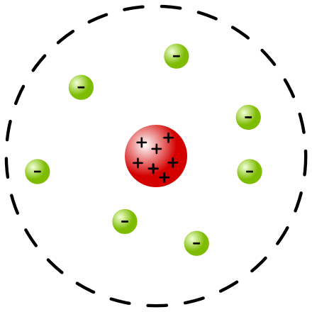
Rutherford’s Nuclear Model of Atom with the nucleus in red and the electrons around it in green colour.

(Source : https://en.m.wikipedia.org/wiki/Rutherford_model)

Moreover, the radiative instability due to electrons being accelerate while orbiting around the nucleus still remained unexplained.

As a result, even though Rutherford had been able to infer the deep structure of atoms on the basis of α-scattering, he, just like Thomson, fell short of explaining the stability of atom.

Bohr’s Model

Absorption of α-particles

Besides the stability of atom, there was another important phenomenon that Thomson and Rutherford could not explain.

It was the absorption of α-particles.

Bohr’s first attempt at atomic modeling was directly influenced by recent work of Charles Galton Darwin on absorption, and Thomson on ionization processes.

Darwin had assumed that the loss of kinetic energy of an α-particle’s when traversing matter was primarily due to encounters with atomic electrons. While, Rutherford had ignored scattering by atomic electrons and was only concerned with the scattering by nucleus.

So, unlike Rutherford, while dealing just with absorption, Darwin did the complete opposite - he ignored the occurrence of large-angle scattering by nucleus, and only focused on scattering by electrons.

Under the right limits, the absorption profiles and scattering formulas he derived were in approximate agreement with experimental data.

Moreover, his final equations depended on only two unknown parameters - the number of electrons in an atom, and the atomic radius.

An Incredulous Bohr

Yet, Bohr thought many of Darwin’s assumptions were objectionable.

So, he decided to work on the problem himself using different methods.

The assumptions he used in deriving his formula for the rate of α-particle absorption made his theory well suited for drawing conclusions from experimental data on the refraction and dispersion of light in hydrogen and helium.

Although, even in 1912, it was still not absolutely clear to physicists that hydrogen contains only a single electron. Using recently compiled data, some physicists were able to deduce that both helium and molecular hydrogen contained about two electrons.

Bohr performed his calculations assuming that both contained exactly two of them.

This led to numbers that were very close to the measured absorption rates of both gases - within 10% for hydrogen and 30% for helium.

He also found substantial agreement for oxygen and several of the heavier elements.

Quantum enters the picture

In 1905, Einstein had applied Max Planck’s quanta in the context of the photelectric effect.

Similarly, Bohr followed suit, applying it in the to atoms.

As per him,

“According to Planck’s theory of radiation we further have that the smallest quantity of energy which can be radiated out from an atomic vibrator is equal to ν.k, where ν is the number of vibrations per second and k = 6.55×10^-27.

This quantity must be expected to be equal to, or at least of the same order of magnitude as, the kinetic energy of an electron of velocity just sufficient to excite the radiation.”

[Bohr 1913a, p. 26-7]

The physical interpretation of Planck’s constant was subject to relentless debate in the decade prior.

Even though it had arisen in a thermodynamic context, namely that of the Blackbody radiation, physicists suspected whether or not it was a purely thermodynamic quantity.

In 1909, Einstein thought there might be some connection between h and the fundamental unit of charge (e). On the other hand, Wien thought that energy quantization was likely due to some kind of universal property of atoms.

Regardless, Niels Bohr was far from being the first to introduce Planck’s ideas into the atomic model.

Haas and Nicholson’s Quantum Mechanical intepretations of the atom

In 1910, Arthur Haas tried to establish links between atomic structure and the numerical value for h.

He proposed to model a neutral hydrogen atom as a uniform sphere of positive charge (radius a) and a single electron (mass m and charge ε) constrained to orbit on the surface of the sphere. For this, he cited a German translation of Thomson’s book “Electricity and Matter”.

The motivation behind this was simply an order of magnitude.

Haas noticed that if he divided h into the energy of an electron at the surface of the atom, the result was of the same order of magnitude as the spectral frequencies for hydrogen.

Therefore, he set hν = (ε^2)/a, where ν is the frequency of both the emitted radiation and the orbital motion of the electron.

Since the electrostatic force between the nucleus and the electron provided the centripetal force, by equating them, Haas found the electron’s orbital frequency ν = ε/2πa sqrt(am) .

This result along with his previous set value for hv led him to an expression for Planck’s constant in terms of other measurable quantities - h = 2επ sqrt(am).

(Solving for a in this equation results would be the same expression for the ground state radius of hydrogen derived by Bohr in 1913.)

Another physicist, J. W. Nicholson, was inspired to use Planck’s ideas in 1912.

He essentially repeated the calculations performed by Thomson in 1904, but for a hypothetical nuclear-type atom called protoflourine (central charge of +5e). This was invented by Nicholson himself to account for certain spectral frequencies in the solar corona.

Based on his calculations, Nicholson offered an alternative view on how Planck’s constant might be related to atoms.

His insight was that the constant could be represented in terms of the total angular momentum of the electrons in their orbit about the nucleus.

“If, therefore, the constant h of Planck has, as Sommerfeld has suggested, an atomic significance, it may mean that the angular momentum of an atom can only rise or fall by discrete amounts when electrons leave or return. It is readily seen that this view presents less difficulty to the mind than the more usual interpretation, which is believed to involve an atomic constitution of energy itself.”

[Nicholson 1912, p. 679]

So, again, unlike popular belief, Bohr wasn’t the one behind the quantization of angular momentum either.

Bohr’s genius

As mentioned earlier, both Thomson and Rutherford’s thories were incapable of explaining the stability of atom.

Bohr was disturbed by both the mechanical and radiative instability inherent to other atomic models. So, he took note of recent work by Nicholson and was appreciative of some of Nicholson’s results. Yet, Bohr was highly critical of any atomic model where the spectral frequencies were equated with electronic orbital frequencies.

This is because any such equivalence would be inconsistent with the discrete nature of spectral lines.

He argued,

’If the “ordinary mechanics” were universally valid, a fixed set of spectral frequencies would require the electrons to orbit at constant speeds for finite amounts of time; but this would be impossible, for as soon as the system started radiating, the orbital frequencies of the charges would begin to change immediately.’

[Bohr 1913b, p. 7]

So, in his seminal paper “On the Constitution of Atoms and Molecules, Part I”, Bohr posited general hypotheses as the basis of his theory :

• The electron is able to revolve in certain stable orbits around the nucleus without radiating any energy (contrary to what classical electromagnetism suggests.) These stable orbits are called stationary orbits and are attained at certain discrete distances from the nucleus. The electron cannot have any other orbit in between the discrete ones.
• The stationary orbits are attained at distances for which the angular momentum of the revolving electron is an integer multiple of the reduced Planck constant mvr = nh/2π

Here, n is called the principal quantum number (then simply called the orbit number).

• Electrons transition between energy states by emitting radiation at a single frequency, which was related to the total emitted energy via Planck’s constant - ΔE = E2 - E1 = hv

The thing that truly distinguished Bohr from his predecessors was not assuming that the spectral frequencies and the orbital frequencies were the same.

Correspondence Principle

Bohr coined the term ‘correspondence principle’ during a lecture in 1920.

Correspondence principle is any one of several premises or assertions about the relationship between classical and quantum mechanics. This principle is called upon by Bohr several times to justify the arguments he makes while putting forth his theory of the Hydrogen atom.

Following his definition of the correspondence principle, Bohr describes two applications :

• The frequency of emitted radiation is related to an integral which can be well approximated by a sum when the quantum numbers inside the integral are large compared with their differences.
• Relationship for the intensities of spectral lines and the rates at which quantum jumps occur

By using his postulates, Bohr obtained that for the hydrogen atom, the energy spectrum approaches the classical continuum for large n (a quantum number that encodes the energy of the orbit)

Hydrogen Spectrum, Balmer formula and the Rydberg Constant

Finally, we come to the most significant of Bohr’s results :

His derivation of the Balmer formula, the Rydberg constant and explaining Hydrogen spectrum in terms of fundamental constants.

Bohr gave us these formulae for the radius, velocity and energy of electron in the ‘nth’ orbit of the electron.

where Z is the atomic number and n is the orbit number (now known as the principal quantum number).

h bar is just h/2π.

The energy difference between states n = n1 and n=n2 for hydrogen can be obtained by putting Z=1 and taking the difference :

As per Bohr’s postulate, this energy difference must be accounted for by the photon released in the process.

So, putting this energy difference equal to hν, we get

For n2 = 2 and integral values of n1 greater than 2 results in the formula discovered by Johann Balmer in 1885 for the visible spectrum of hydrogen.

The family of frequencies corresponding to these electronic transitions is thus called the Balmer series. Similarly, n2 = 3 corresponded to the infrared spectrum (Paschen series) observed by Paschen in 1908. The series corresponding to n2 = 1, 4, 5… were then, yet to be observed as they were either in extreme UV (for n2 = 1), or extreme Infrared (for n2 = 4, 5…).

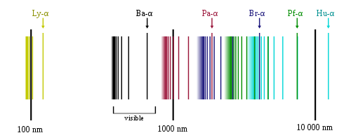
Hydrogen Emission Spectrum showing Lymann, Balmer, Paschen, Brackett, Pfund and Humphrey series.

(Source : https://en.m.wikipedia.org/wiki/Hydrogen_spectral_series)

The Balmer formula was known for decades, but had hitherto no theoretical explanation.

Throughout his life, Bohr claimed that he had been unaware of Balmer’s empirical formula until he was already well along in the development of his theory.

Bohr achieved what Thomson and Rutheford couldn’t. He made the theory of Hydrogen spectrum agree with the experimental observations. And he did so while deriving the Balmer formula and the Rydberg constant.

This single derivation, made Bohr the legend we know him as today.

References

• Early Atomic Models - From Mechanical to Quantum (1904-1913) by Charles Baily
• https://en.m.wikipedia.org/wiki/Vortex_theory_of_the_atom
• https://en.m.wikipedia.org/wiki/Hantaro_Nagaoka
• https://en.m.wikipedia.org/wiki/Bohr_model
• https://en.m.wikipedia.org/wiki/Correspondence_principle